7 concepts20 worked examples29 exercises5 exam-level7 figures
What are you here for?
13 Understanding experimental data: the least squares line, polyfit and polyval, the number that says how good a fit is, and why a better fit can be a worse model
Start with this
One question before you read anything. Getting it wrong is the point: it shows you what this section is for.
§13.0 — a data line split into pieces
One line of a measurement file, split on the space. Nothing about fitting yet: this is only about what split hands back. If you do not know the second line, read the answer, that is what it is for.
Find(a) Write exactly what this program prints, all four lines.
Given
line = '0.0865 0.1'
parts = line.split(' ')
print(parts)
print(parts[0] + parts[1])
print(float(parts[0]) + float(parts[1]))
print(len(parts), type(parts[0]))
IPython console
In [1]: %run untitled0.py
The second line is the whole reason float appears in every file reading function in this course. Nothing was added there: two pieces of text were glued together, and the result is a string that looks almost like a number.
Hint 1/4
Decide what kind of thing split puts in the list before you decide what the plus sign does.
Hint 2/4
split returns a list of strings, always. Plus on two strings joins them; plus on two floats adds them.
Hint 3/4
The line is '0.0865 0.1', so the list is ['0.0865', '0.1']. Line two joins those two pieces of text. Line three converts first, then adds.
Hint 4/4
The list, then the joined text, then the sum, then the length and the type of a piece.
Show solution
Tracking the type is cheaper than tracking the value here, because every surprise in this program comes from a type and none from arithmetic.
Split the line
$$\texttt{parts} = \texttt{['0.0865', '0.1']}$$
split cuts at the space and keeps both pieces as text
The joined string has 9 characters, which is the 6 of the first piece plus the 3 of the second; a real addition could not have produced a longer text than either operand.
Every measurement that comes from a file is text until something converts it. Convert at the moment of reading, not later.
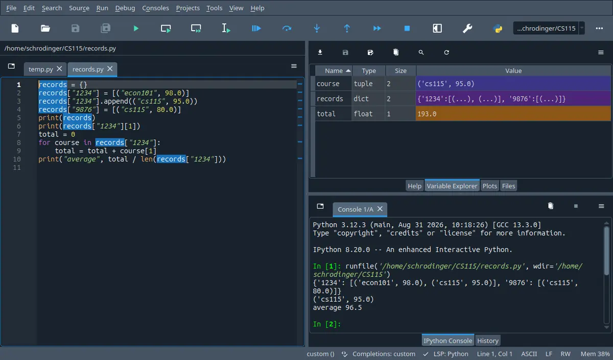
What this looks like in Spyder
The tab next to Help. It lists every name your program left behind with its type and its size, so it answers the one question a listing cannot: what is in this name right now. The stepper on this page shows the same four columns.
Spyder 5.5.1 on Linux, running the program in its own editor. A different version moves a few toolbar icons; the panes are named the same.
A spring hangs from a hook. You add a weight, measure how much longer the spring got, and write the pair down.
Thirteen rows later, the theory still promises one number for this spring. Worked out row by row it gives thirteen, the smallest 11.34 and the largest 19.18.
Nothing in the rows says which to believe.
By the end of this section you can turn a file of measurements into one line, read the physical constant off that line, print a score that says how much of the data the line accounts for, and say when a curve that fits better is the worse answer.
In 60 seconds
Measurements land around the theory's line and not on it, so you fit one line to all the points at once, read what you wanted off the fit, and report one number that says how much of the spread the fit accounts for.
When the quantity you want is not the fit itself but something the fit's slope contains. For the thirteen rows here the slope is 0.064711, so k is 15.45 newtons per metre.
Reporting a fit. 1 means the model passes through every point, 0 means it is no better than the flat average, and a negative value means it is worse than that.
Three most common mistakes
Building the predicted list by writing predicted = observed, which gives one list two names and silently turns every gap into zero.
Sorting one of the two measurement lists, which keeps the numbers and destroys the pairing between them.
Reading a rising R squared as a better model. Every extra degree raises it on the points that were fitted, all the way to 1.
The syllabus splits the mark as labs 20, midterm 40 and final 40. In the course plan this material sits in the last weeks, after the midterm week, so it is final material and lab material, not midterm material.
How much time do you have?
10 minutes
What a fit is scored on, the two calls that produce one, and the four boxed results. Enough to read a fitting program and say what each line is for.
The 60-second card · What best means: the sum of squared gaps · The line the data picks · Formula card
45 minutes
Enough to write the fit and the score from scratch in plain Python, to trace someone else's version without running it, and to answer the question exams ask about degree: which fit do you report.
The 60-second card · The predicted list · The line the data picks · How good the fit is · A better fit on the same points can be a worse model · Method boxes · B · computation
full read
The whole path from a text file of measurements to a defended answer: one line, one physical constant, one score, and one sentence about the range the answer is good for.
The 60-second card · Recall first · Conventions · Measurements land around the theory, not on it · What best means: the sum of squared gaps · The predicted list · The line the data picks · How good the fit is · What the fit is good for · A better fit on the same points can be a worse model · Scaffolding comes off · Full exam-style question · Practice set · Mistake ledger
By the end of this section
Explain why measurements sit around a model rather than on it, and compute the residual at one point.
Compute the sum of squared gaps for a candidate model and use it to pick between two candidates.
Write the loop that builds a predicted list without disturbing the measured lists or their pairing.
Produce the line for a set of measurements, both from the two sums formula and with polyfit and polyval.
Report the coefficient of determination for a fit and say what its value does and does not promise.
Bound a fitted result to the range of the measurements and show what refitting a subset does to a physical constant.
Choose the by scoring it on measurements it was not fitted to, and explain why the fitted score alone cannot decide.
Syllabus coverage
covered
Understanding Experimental Data — covered
The whole path the week names: an experiment produces paired measurements, a theory says what shape they should have, a program fits that shape to the points, and a second number says how well it fits. The spring experiment and its thirteen rows carry all of it, from the residual at one point to the choice of degree.
covered
Chapter 18 — covered
The chapter parts this page uses: springs and the , the least squares objective, polyfit and polyval, the coefficient of determination, what a rising degree does to it, and the case where no theory fixes the shape. The chapter's one transformation trick, fitting a line to the logarithm, is here as a single worked example.
off syllabus
loadtxt and arrays as the container measurements arrive in — off syllabus
The tenth lab reads its data file into an array and slices columns out of it, rather than appending to two lists.
Not named in this week's syllabus line. It is here in two sentences because the lab paper reads its file that way, and a student who has only seen the two list version reads the array version as another language. The fitting calls take both.
off syllabus
scoring a fit on measurements it was not fitted to — off syllabus
Splitting the rows, fitting one part and scoring the other, with the numbers that come out of this data set.
The syllabus line names no method for this. The numbers force it: on the rows a model was fitted to, the score rises with every extra degree, up to a perfect 1. Without a second set of rows nothing shows that the model got worse. Shown as the cheapest honest check, not as a named technique.
Recall first
A file, line by line, into numbers
open(name, 'r'), one readline() to swallow the header, then for line in dataFile: with d, m = line.split(' ') and float(d). The data file for this week has a header row and two columns separated by a space.
The measurements this page fits arrive as text. split hands back strings, and adding two of those concatenates them instead of adding them.
Building a list with append, indexing with range
values = [] then values.append(x) inside a loop. To walk two lists together, for i in range(len(xs)): and use xs[i] and ys[i].
Every predicted list on this page is built this way, and the paired index is what keeps a measurement next to its own prediction.
The average of a list
Add the items in a loop, then divide by len(values). With / it is a float; with // it is a floor, which for a list of measurements under 1 is 0.0.
The score for a fit compares the model's error against the spread of the measurements around their own average, so the average is inside the formula.
Two series in one panel, with a legend
plot(xs, ys, 'ro') for markers only, plot(xs, predicted) for a plain line, then legend(['measured', 'fit']), plus title, xlabel and ylabel.
A fit is reported as a picture with the measurements still visible. The markers are the data, the line is the model, and the legend is what tells them apart.
The mean of many runs as the reported answer
One run of a process answers nothing; the reported number is the average over many runs, quoted with its spread.
The same habit applies to one measurement here. Thirteen rows are thirteen runs of the same experiment, and the fit is what replaces them with one answer.
Try it yourself first (2 questions)
1§13.0 — two lists walked with one index
Four rows of the spring data, as two lists in the same order. The program turns each mass into a force and then prints the ends of both lists.
Find(a) Write exactly what this program prints, all three lines.
Each force is about ten times its mass, which is what multiplying by 9.81 should do, and the list is still increasing, like the masses.
A derived list built with append inherits the order of the list it came from, which is why a shared index keeps working.
2§13.0 — the average of gaps that cancel
Four gaps between measurement and model, two of them positive and two negative. The program adds them, averages them, and then adds their squares. This is the trap this section is built on, so being wrong here costs nothing.
Find(a) Write exactly what this program prints, all three lines.
Given
gaps = [0.02, -0.01, 0.03, -0.04]
total = 0for i inrange(len(gaps)):
total = total + gaps[i]
print(round(total, 4))
print(round(total / len(gaps), 4))
squared = 0for i inrange(len(gaps)):
squared = squared + gaps[i] ** 2print(round(squared, 4))
IPython console
In [1]: %run untitled0.py
Four gaps of up to 0.04, and the total says the model is perfect. That is the whole argument for squaring: the first two lines cannot tell a good model from a bad one, and the third can.
Hint 1/4
Add the four signed numbers first, and only then ask what the third print measures instead.
Hint 2/4
A sum of signed numbers can be zero while none of them is zero. Squares are never negative, so a sum of squares is zero only when every item is.
Hint 3/4
The gaps are 0.02, -0.01, 0.03 and -0.04. Their sum is 0.02 - 0.01 + 0.03 - 0.04. Their squares are 0.0004, 0.0001, 0.0009 and 0.0016.
Hint 4/4
The first two lines are the same number, and the third is not.
Show solution
Do the signed sum by pairing the positives against the negatives; it is faster than left to right and it shows immediately why the answer is 0.
grouping by sign shows the cancellation instead of hiding it in the running total
$$0.05 - 0.05 = 0.0$$
so the total, and therefore the average, are both 0.0
Add the squares
$$0.0004 + 0.0001 + 0.0009 + 0.0016 = 0.003$$
squares of the same four numbers, all positive, so nothing can cancel
Answer $$\boxed{0.0 \;/\; 0.0 \;/\; 0.003}$$
Check
The largest gap is 0.04 and its square alone is 0.0016, which is over half the total, so a total of 0.003 is the right order of magnitude.
Any measure of fit has to be blind to the sign of a gap. Squaring is the cheapest way to arrange that.
Notation
symbol
reads as
means
watch out
$observed, predicted$
the measured values and the model's values
Two lists of the same length, in the same order. observed[i] came out of the experiment, predicted[i] came out of the model at the same x.
Same length and same order is the whole contract. Sort one of them and every pair after the first is wrong, with no error raised.
$residual$
observed minus predicted
The signed gap at one point. Positive means the measurement is above the model, negative means below.
Signed. Adding residuals up is close to meaningless because they cancel; the sum of their squares is what gets used.
$polyfit(xs, ys, n)$
fit a polynomial of degree n to these points
Hands back n+1 coefficients as an array, highest power first. Degree 1 gives [slope, intercept].
The x list comes first. polyfit(ys, xs, 1) fits the axes the other way round, returns two plausible numbers and raises nothing.
$polyval(fit, xs)$
evaluate this polynomial at these x values
Takes the from polyfit plus one x or a whole array of them, and returns the model's y for each.
The coefficients come first, the x values second. The order inside the coefficient array is highest power first, which is the opposite of what most people write on paper.
$k$
the spring constant
Newtons per metre. A stiff spring has a large k. In this data the fit's slope is metres per newton, so k is one over the slope.
It is one over the slope, not the slope. Reporting 0.0647 newtons per metre for a spring that takes 15.45 newtons to stretch a metre is a factor of 239 out.
$R squared$
the coefficient of determination
One minus the fit's squared error divided by the squared spread of the measurements around their own average.
It has no units and it is not a percentage of anything you measured. On points the model was not fitted to it can go below zero.
Conventions used here
Which lab this is for, and which library does which half.
This page is written for the tenth lab, the plotting lab, whose data question puts a fitted line through a file of measurements.
The split is clean: numpy fits with polyfit and polyval, matplotlib draws.
Both import styles the course uses appear in its files: from numpy import * next to import numpy as np. Pick one per file.
A student who looks for a separate fitting lab does not find one, and concludes the material is not practised. It is practised inside the plotting lab, where the fit is two lines in the middle of a drawing question.
Where the printed numbers on this page came from.
Every console block here is a real run, pasted as it came out.
The plain Python fitting programs were run as printed. numpy's polyfit returns 0.064711 and 0.003336 for this data, which agrees with the plain Python function to six decimal places.
The pictures are drawn from those numbers.
In a programming course the printed answer is the claim. A page that shows a made up coefficient teaches a wrong number that a student then defends in a lab.
How numbers are rounded, and how they are compared.
Fitted coefficients are reported with round(value, 6), scores with round(value, 4). The raw values carry seventeen digits that mean nothing about a spring measured to four.
Two floats are never compared with == here. The test is abs(a - b) < 0.0001.
A rounded number is for reading. Keep the unrounded one for the next calculation.
0.1 + 0.2 == 0.3 is False in Python, and a fit compares computed values to measured ones at every point. An equality test between them is a test that always fails.
The words for the three quantities, and the one that is not a mistake.
observed is what the experiment gave. predicted is what the model gives at the same x. residual is observed minus predicted, with its sign.
The squared sum of residuals is the error of the fit. A perfect program on perfect data still has one.
An is a point far from the fit; it stays unless you can say why.
The word error carries two meanings in this week's material, and a student who reads the fit's error as a bug goes looking for a bug that is not there.
The sign in Hooke's law and the magnitudes in the data.
The law is written with a minus sign, force and displacement pointing opposite ways. The data file records magnitudes, both positive.
So the fitted numbers are force = mass * 9.81 against distance, and the slope comes out positive.
The lecture material labels that axis with absolute value bars for this reason.
A student who fits the law as written gets a negative slope and a negative spring constant, then cannot tell whether the sign is the physics or a bug in the program.
Units, kept on the page and out of the program.
Distance is in metres, mass in kilograms, force in newtons, and k in newtons per metre.
The programs carry bare floats, so the units live in the print strings and in the axis labels. 9.81 is metres per second squared, which is what turns a mass into a force.
A fit of unlabelled columns is a number without a meaning.
The lab data files are columns of bare numbers. The only place the unit can be recorded is the label you write, and an unlabelled axis is the most common mark lost in a plotting lab.
13.1Measurements land around the theory, not on it
The useful object is not a measured point but the signed gap between that point and what the model says.
The plotting section put the measurements on the screen. The question now is what to draw through them, and why anything has to be drawn at all.
Solvable with what we have
Read a two column data file into two lists of floats.
Turn each mass into a force with masses[i] * 9.81.
Draw the pairs as red circles with labelled axes.
Not solvable yet
Report the one spring constant the theory promises.
Predict the stretch under a load nobody measured.
Choose between two candidate lines through the cloud.
Hooke's law says the stretch is proportional to the force, so every row on its own should give the constant. Divide force by distance, thirteen times, and the first worked example below runs it.
Why it fails
Thirteen rows give thirteen constants, from 11.34 to 19.18. Averaging them is a guess: it weights the lightest row as heavily as the heaviest. Nothing in the thirteen numbers says which to believe.
The residual at a point is the measurement minus what the model says there. Positive means the measurement is above the model, negative means below, and zero means the model passes exactly through that point.
The thirteen rows with a straight line through them. The purple segments are the residuals: one per row, signed, and the longest of them is 0.0465 metres at the 0.45 kg row. The line is not near the points because the spring is odd, it is near them because no line can be nearer.
Looks like this, but is not
A model with no residuals at all is easy to build: join the measured points to each other.
plot(forces, distances)
Every measured point is on it, so every residual is zero.
It has no slope to report, so there is no spring constant in it. Between two rows it predicts whatever the line segment happens to say, and its kinks are measurement noise drawn as if it were physics.
row
mass (kg)
force (N)
distance (m)
0
0.10
0.9810
0.0865
1
0.15
1.4715
0.1015
2
0.20
1.9620
0.1106
3
0.25
2.4525
0.1279
4
0.30
2.9430
0.1892
5
0.35
3.4335
0.2695
6
0.40
3.9240
0.2888
7
0.45
4.4145
0.2425
8
0.50
4.9050
0.3465
9
0.55
5.3955
0.3225
10
0.60
5.8860
0.3764
11
0.65
6.3765
0.4263
12
0.70
6.8670
0.4562
Row 7 measured less than row 6 even though it carried more weight, and rows 8 and 9 do the same. The column is not monotonic, and no straight line can make it so.
Thirteen rows, thirteen spring constants, and a hand check of the worst one
Row by row, the constant is the force divided by the measured stretch.
This program does that thirteen times and reports the two extremes:
rows: 13
k from each row: [11.34, 14.5, 17.74, 19.18, 15.55, 12.74, 13.59, 18.2, 14.16, 16.73, 15.64, 14.96, 15.05]
smallest: 11.34 largest: 19.18
Row 3 is the 0.25 kg mass with a stretch of 0.1279 m, and the run printed 19.18 for it. Confirm that number by hand, then say what it would take for it to be the spring's constant.
FindThe constant this one row implies, and whether one row can settle it.
Given
mass 0.25 kg, distance 0.1279 m
force = mass times 9.81
the printed value for this row: 19.18
Solution
Recomputing the extreme row is cheaper than checking all thirteen, and if the extreme one is right the rest of the list is almost certainly right too.
Turn the mass into a force
$$F = 0.25 \cdot 9.81 = 2.4525\ \text{N}$$
the file records a mass, and Hooke's law is about the force it applies
Divide by the measured stretch
$$k = \frac{2.4525}{0.1279} = 19.175\ldots$$
this row alone, treated as if it had no
$$\boxed{k \approx 19.18\ \text{N/m}}$$
rounded the way the program rounds it, so the two agree
Answer $$\boxed{k \approx 19.18\ \text{N/m from this row alone}}$$
Check
Row 12 gives 6.867 divided by 0.4562, which is 15.05. Two rows of one spring cannot both be right, so at least one of them carries measurement error, and there is no reason it is only one.
One multiplication and one division per row, and thirteen answers at the end of it.
A single measurement, divided, is a constant with an unknown error attached. The fix is not a better row, it is using all of them at once.
The residual at the 0.45 kg row
Take the line this data picks, slope 0.064711 and intercept 0.003336, and find the signed gap at the 0.45 kg row, whose measured stretch is 0.2425 m.
This program walks all thirteen rows and prints the row number, the model's value and the gap:
00.06680.019710.09860.002920.1303 -0.019730.162 -0.034140.1938 -0.004650.22550.04460.25730.031570.289 -0.046580.32070.025890.3525 -0.03100.3842 -0.0078110.4160.0103120.44770.0085
largest gap at row 7 size -0.0465
FindThe predicted stretch and the residual at that row.
Given
slope 0.064711, intercept 0.003336
the 0.45 kg row: force 4.4145 N, measured distance 0.2425 m
Solution
Computing the one row by hand and reading the rest from the run is cheaper than hand computing thirteen, and it checks the program at the same time.
Ask the model
$$0.064711 \cdot 4.4145 = 0.285575$$
the slope times this row's force
$$0.285575 + 0.003336 = 0.288911$$
plus the intercept, which the run prints as 0.289
Subtract in the right order
$$0.2425 - 0.2889 = -0.0464$$
observed minus predicted, so a measurement below the model is negative
The neighbouring rows at 3.924 N and 4.905 N measured 0.2888 and 0.3465. This row measured less than the lighter one did, so a large negative gap is what the numbers demand.
Thirteen residuals, one multiplication and one subtraction each.
The sign of a residual says which side of the model the measurement fell on, and that is the information a later step will throw away deliberately.
Checkpoint
§13.1 — reading a residual
A model says a rod at 40 degrees will be 1.204 m long. The rod is measured at 1.198 m. The lab report has to record the residual.
Find(a) Which value goes in the residual column?
Given
predicted 1.204 m
observed 1.198 m
Hint 1/4
Decide which of the two numbers is the measurement and which is the model before subtracting anything.
Hint 2/4
The residual is observed minus predicted, in that order, and it keeps its sign.
Hint 3/4
Observed is the measured 1.198 m, predicted is the model's 1.204 m, so the subtraction is 1.198 minus 1.204.
Hint 4/4
The measurement is below the model, so the answer is negative and small.
Show solution
Substituting into the definition is the whole task here; any rearranging is a chance to swap the order.
Substitute
$$1.198 - 1.204 = -0.006$$
observed first, predicted second, as the definition fixes it
Answer $$\boxed{-0.006\ \text{m}}$$
Check
The magnitude is 6 mm out of 1.2 m, about half a percent, which is the order of magnitude a length measurement error should have.
Every later formula on this page squares this number, so the sign matters here and nowhere after.
⚠ Averaging the per row constants and calling it the answer
Thirteen numbers and a mean is a habit from the trials section, where the runs really were interchangeable.
Go through the points one at a time, take the gap between the measurement and the model, square it so the sign cannot cancel, and add. The model with the smaller total is the better fit on these points.
Four gaps, on the left with their signs and on the right squared. The signed total is 0.0, which would call this model perfect. The squared total is 0.003, and the largest single gap contributes 0.0016 of it, over half.
Looks like this, but is not
Adding the signed gaps looks like the same idea and is one character shorter:
total = total + (observed[i] - predicted[i])
The flat line through the average of the measurements makes that total exactly zero, and so does any line through the middle of the cloud. A score that a bad model can reach is not a score.
Two candidate lines on the spring data, scored
One person proposes distance = 0.06 times force. Another proposes 0.0575 times force plus 0.0055. Both look reasonable on the picture. Score them.
The program builds each model's predicted list and adds the squared gaps:
defpredict(slope, intercept, xs):
"""Return the model's value at every x in xs."""
out = []
for i inrange(len(xs)):
out.append(slope * xs[i] + intercept)
return out
defsum_of_squares(observed, predicted):
"""Add up the squared gap at every point."""
total = 0for i inrange(len(observed)):
total = total + (observed[i] - predicted[i]) ** 2return total
forces = [0.981, 1.4715, 1.962, 2.4525, 2.943, 3.4335, 3.924,
4.4145, 4.905, 5.3955, 5.886, 6.3765, 6.867]
distances = [0.0865, 0.1015, 0.1106, 0.1279, 0.1892, 0.2695, 0.2888,
0.2425, 0.3465, 0.3225, 0.3764, 0.4263, 0.4562]
first = predict(0.06, 0.0, forces)
second = predict(0.0575, 0.0055, forces)
print('line A loses', round(sum_of_squares(distances, first), 6))
print('line B loses', round(sum_of_squares(distances, second), 6))
line A loses 0.016027
line B loses 0.020018
FindWhich line fits these points better, and by how much.
Given
line A: slope 0.06, intercept 0.0
line B: slope 0.0575, intercept 0.0055
the thirteen rows of the spring data
Solution
Two functions rather than one loop, because the predicted list is needed again later for the score and for the picture; a single fused loop would have to be written twice.
Score line A
$$\text{SSE}_A = 0.016027$$
thirteen squared gaps, added by the loop
Score line B and compare
$$\text{SSE}_B = 0.020018$$
same points, same procedure, so the two numbers are comparable
$$\boxed{\text{A wins},\ 0.016027 < 0.020018}$$
lower total means smaller gaps overall, which is what better fit means here
At the heaviest row, 6.867 N, line A says 0.4120 and line B says 0.3954 against a measurement of 0.4562. A is closer there, and the ranking agrees with the totals.
Two passes of thirteen points each, so 26 subtractions and 26 squarings.
The winner of a comparison is only the winner among the candidates offered. Neither of these is the best line, and the next concept produces the one that is.
A model with four gaps and a perfect signed total
Four measurements, and a model that is 0.05 too high at two points and 0.05 too low at two others. Score it both ways and see which score can tell.
observed = [0.10, 0.20, 0.30, 0.40]
predicted = [0.15, 0.15, 0.35, 0.35]
signed = 0
squared = 0for i inrange(len(observed)):
gap = observed[i] - predicted[i]
signed = signed + gap
squared = squared + gap ** 2print('sum of gaps:', round(signed, 4))
print('sum of squared gaps:', round(squared, 4))
sum of gaps: 0.0sum of squared gaps: 0.01
FindBoth totals, and what each one claims about the model.
Given
observed 0.10, 0.20, 0.30, 0.40
predicted 0.15, 0.15, 0.35, 0.35
Solution
One loop that accumulates both totals, because the comparison is the point and two separate loops would let the two numbers drift apart in the reader's head.
Collect the four gaps
$$-0.05,\ +0.05,\ -0.05,\ +0.05$$
observed minus predicted at each of the four points, in order
Add them, then add their squares
$$\text{signed total} = 0.0$$
the two negatives cancel the two positives exactly
Every point is 0.05 from the model, so a correct squared total has to be four times 0.0025. It is, and a signed total of 0.0 therefore cannot be reporting on the same four gaps.
Any score that lets positive and negative errors meet is a score a wrong model can pass.
Checkpoint
§13.2 — scoring a model on three points
Three measurements and one model, small enough to do in your head. The score is the one from the box above.
Find(a) Compute the sum of squared gaps for this model.
Given
observed: 2.0, 4.0, 6.0
predicted: 2.1, 3.8, 6.3
Hint 1/4
Write the three gaps down first, with their signs, and do not add anything yet.
Hint 2/4
Each term is observed minus predicted, squared. The signs disappear only after the squaring.
Hint 3/4
The pairs are 2.0 against 2.1, 4.0 against 3.8 and 6.0 against 6.3, so the gaps are -0.1, +0.2 and -0.3.
Hint 4/4
Three squares to add, and the largest of them is more than half the total.
Show solution
Squaring before adding is not optional bookkeeping here; adding first would give -0.2 and hide two of the three errors.
Start from an empty list, and for each measured x append the model's value for that x. When the loop ends the two lists have the same length and the same order, which is exactly what the score assumes.
The same two names in two situations. Above, one list with two names: writing into predicted[0] changes observed[0] too, and every gap comes out 0.0. Below, predicted = [] and one append per point, so the measured list is still the measured list.
Looks like this, but is not
This looks like the cheapest way to get a list of the right length:
predicted = observed
for i inrange(len(predicted)):
predicted[i] = slope * xs[i] + intercept
It never makes a second list. Both names reach the same object, so the assignment overwrites the measurements as it goes, and every residual computed afterwards is exactly zero. The score then reports a perfect fit for any slope at all.
What predicted = observed does to the gaps
This is the bug with the smallest possible data set. Three measurements, a model written into the wrong list, and three gaps that all come out zero.
observed = [0.10, 0.20, 0.30]
predicted = observed
for i inrange(len(predicted)):
predicted[i] = 0.15 + 0.05 * i
gaps = []
for i inrange(len(observed)):
gaps.append(round(observed[i] - predicted[i], 2))
print(observed)
print(predicted)
print(gaps)
FindWhat the three prints show, and where the measurements went.
Given
observed starts as 0.10, 0.20, 0.30
the model writes 0.15, 0.20, 0.25 into predicted
Solution
Printing both lists rather than only the gaps, because a list of zeros looks like a perfect fit and only the first line proves the measurements are gone.
Follow the assignment
$$\texttt{predicted = observed}$$
one list, two names; nothing was copied, so there is nothing to write into separately
Run it with the model 0.90 plus 0.05 times i instead. The gaps are still all 0.0, which no real model could manage on this data, so the zeros are coming from the aliasing and not from the model.
A fit that scores perfectly on the first try is a reason to print both lists before believing it.
Sorting one list of a pair
The rows arrived out of order, so sorting looks like tidying. This program sorts the masses and leaves the distances alone.
masses = [0.3, 0.1, 0.2]
distances = [0.1892, 0.0865, 0.1106]
masses.sort()
print(masses)
print(distances)
for i inrange(len(masses)):
print(masses[i], distances[i])
index 0 of one list with index 0 of the other, as every loop on this page does
$$\boxed{\text{all three pairs are wrong}}$$
the true pairs were (0.3, 0.1892), (0.1, 0.0865) and (0.2, 0.1106)
Answer $$\boxed{\text{three pairs, none of them measured}}$$
Check
The lightest mass is now paired with the largest stretch, which is the opposite of what the spring does, so the pairing is provably scrambled and not merely suspicious.
If the rows have to be ordered, sort an index list or build pairs first. Sorting half of a pair destroys data without raising anything.
The predicted list, built the way the rest of the page uses it
Four rows of the spring data and the line this data picks. The function returns a new list and touches nothing.
defpredict(slope, intercept, xs):
"""Return the model's value at every x in xs."""
out = []
for i inrange(len(xs)):
out.append(round(slope * xs[i] + intercept, 4))
return out
forces = [0.981, 1.4715, 1.962, 2.4525]
distances = [0.0865, 0.1015, 0.1106, 0.1279]
fitted = predict(0.064711, 0.003336, forces)
print('measured :', distances)
print('predicted:', fitted)
print('first gap:', round(distances[0] - fitted[0], 4))
FindThe predicted list, and the gap at the first row.
Given
four forces: 0.981, 1.4715, 1.962, 2.4525
slope 0.064711, intercept 0.003336
Solution
The function takes the x list and returns a new one, so it can be called for the measured x values and again for a drawing grid without either call disturbing the other.
Build the new list
$$\texttt{out = []}$$
a fresh list, so nothing the caller owns can be written into
$$0.064711 \cdot 0.981 + 0.003336 = 0.0668$$
the first append, rounded to four places for printing
Take one gap
$$0.0865 - 0.0668 = \boxed{0.0197}$$
measured above the model at the lightest weight, so the gap is positive
Answer $$\boxed{\texttt{[0.0668, 0.0986, 0.1303, 0.162]}, \quad \text{first gap } 0.0197}$$
Check
The measured list is printed after the call and is unchanged, and the rise by about 0.0317 per row, which is the slope times the 0.4905 N step between rows.
One multiplication, one addition and one append per point.
A function that returns a new list can be called twice without a second thought, which is why every later step on this page calls this one.
Checkpoint
§13.3 — which line damages the measurements
A student wants a list of model values with the same length as the measurements. Four candidate first lines, one program.
Find(a) Which first line leaves the measurements intact and still lets the loop write?
Given
observed holds the measurements
the loop that follows writes into predicted[i] for every i
Hint 1/4
Ask of each candidate how many list objects exist after it runs.
Hint 2/4
Assignment between names never copies a list. A new list comes from [], from a slice, or from list(...).
Hint 3/4
The loop writes into predicted[i] for every i, so whatever object that name reaches is the object that gets changed.
Hint 4/4
Only one candidate creates a second object, and it needs append rather than indexed assignment.
Show solution
Counting objects settles all four candidates at once, where tracing each program separately would take four traces.
Collect four running sums as you walk the points: the x values, the y values, the squares of the x values, and the products x times y. The slope is built from all four, and the intercept then forces the line through the point where the two averages meet.
What the array from polyfit means. Position decides the power, and the highest power is first, so a degree 2 fit hands back three numbers with the constant last. Reading the array backwards is the commonest way to get a plausible and wrong curve.
Looks like this, but is not
The two lists are both measurements, so the order of the arguments looks like a matter of taste:
fit = polyfit(distances, forces, 1)
It fits force against distance, which is a different question. On this data it returns a slope of 14.74, and one over that is 0.0678, not the 0.0647 the right way round gives. Both are plausible numbers and nothing is raised.
The spring's line and its spring constant, in plain Python
Everything the fit needs is in four sums. The function collects them in one pass, applies the rule, and the caller turns the slope into a physical constant.
slope: 0.064711
intercept: 0.003336
spring constant: 15.45 newtons per metre
FindThe slope, the intercept, and the spring constant they imply.
Given
the thirteen forces, from mass times 9.81
the thirteen measured distances
Solution
One pass collecting four sums, rather than four passes collecting one each: the loop body is longer but the data is walked once, which is the habit the complexity section argued for.
Collect the four sums
$$n = 13, \quad \sum x = 51.0120, \quad \sum y = 3.3444$$
the x values are forces in newtons and the y values are metres
$$\sum x^2 = 243.9585, \quad \sum xy = 15.9569$$
the two sums that carry the shape of the cloud rather than its position
The per row constants ran from 11.34 to 19.18 and their middle rows sat near 15. A fitted 15.45 lands inside that range, which a mistake in the sums would not be obliged to do.
One pass over thirteen points, four multiplications and four additions per point.
The fit is two numbers. Everything after this, the score, the picture and the physics, is read off those two.
The same fit as the lecture files write it, with polyfit and polyval
The course does not write the four sums. It calls numpy, and the whole fit is two lines in the middle of a drawing function.
This is the shape the lab expects, reading a file and putting the model on top of the measurements:
from matplotlib.pyplot import *
from numpy import *
deffit_data(input_file):
"""Draw the measured points and the least squares line through them."""
masses, distances = get_data(input_file)
forces = []
for i inrange(len(masses)):
forces.append(masses[i] * 9.81)
plot(forces, distances, 'ro', label='measured displacements')
fit = polyfit(forces, distances, 1)
predicted = polyval(fit, forces)
plot(forces, predicted, label='displacements predicted by the linear fit')
title('Measured displacement of spring')
xlabel('force (newtons)')
ylabel('distance (metres)')
legend(loc='best')
Run on these thirteen rows, fit holds 0.064711 and 0.003336, the same two numbers the plain Python function printed, and polyval at the first force gives 0.066817.
FindWhich line does the fitting, which does the predicting, and what the returned array holds.
Given
the data file with a header row and two columns
polyfit(xs, ys, 1) for the coefficients and polyval(fit, xs) for the predicted values
Solution
polyval rather than a loop over the coefficients, because the same call works unchanged when the degree changes and a hand written a*f + b does not.
Separate the fitting from the drawing
$$\texttt{fit = polyfit(forces, distances, 1)}$$
the only line that looks at both lists together and produces the model
$$\texttt{predicted = polyval(fit, forces)}$$
the model evaluated at the measured x values, which is what gets drawn and scored
The plain Python function on the same thirteen rows printed 0.064711 and 0.003336. Two independent routes to six matching decimal places is the check that the sums were collected correctly.
Two calls instead of a fifteen line function, and the degree becomes a single argument.
Learn the four sums so the two calls are not magic, then use the two calls.
A curve a straight line can still fit: take the logarithm first
Not every theory predicts a straight line. If y multiplies by a constant factor every time x goes up by one, the straight line is in the logarithm.
This program takes the log of each measurement and fits a line to that:
import math
deffit_line(xs, ys):
"""Return the slope and intercept of the least squares line."""
n = len(xs)
sum_x = 0
sum_y = 0
sum_xx = 0
sum_xy = 0for i inrange(n):
sum_x = sum_x + xs[i]
sum_y = sum_y + ys[i]
sum_xx = sum_xx + xs[i] * xs[i]
sum_xy = sum_xy + xs[i] * ys[i]
slope = (n * sum_xy - sum_x * sum_y) / (n * sum_xx - sum_x * sum_x)
intercept = (sum_y - slope * sum_x) / n
return slope, intercept
xs = [0, 1, 2, 3, 4, 5]
ys = [3, 6, 12, 24, 48, 96]
logs = []
for i inrange(len(ys)):
logs.append(math.log(ys[i]))
a, b = fit_line(xs, logs)
print('slope of the log fit:', round(a, 6))
print('intercept of the log fit:', round(b, 6))
print('log of 2:', round(math.log(2), 6))
print('log of 3:', round(math.log(3), 6))
slope of the log fit: 0.693147
intercept of the log fit: 1.098612
log of 2: 0.693147
log of 3: 1.098612
FindWhat the fitted line in log space says about the original data.
Given
x from 0 to 5
y doubling each step: 3, 6, 12, 24, 48, 96
Solution
Fitting the log rather than a high degree polynomial: the polynomial would score well on these six points and would still not contain the doubling, which is the thing worth reporting.
Fit the transformed data
$$\text{slope} = 0.693147$$
the run prints it, and the next lines of the run name it
$$\text{intercept} = 1.098612$$
the value of the log fit at x equals 0
Read the two numbers back into the original data
$$0.693147 = \ln 2$$
the program prints the log of 2 on the next line for exactly this comparison
$$1.098612 = \ln 3$$
so the fit says y is 3 times 2 to the power x
$$\boxed{y = 3 \cdot 2^{x}}$$
a factor per step and a starting value, recovered from a straight line fit
Answer $$\boxed{y = 3 \cdot 2^{x}, \ \text{read off as } \ln 2 \ \text{and} \ \ln 3}$$
Check
Put x equal to 5 into the recovered model: 3 times 32 is 96, which is the last measurement exactly.
One extra list of logarithms, and the same fitting function as everything else on this page.
When the theory says factor per step, fit the logarithm. The slope is then a growth rate, not a distance per newton.
Checkpoint
§13.4 — reading a coefficient array
A fit was run and the coefficient array printed as [2.5, -1.0, 0.5]. The next line of the program needs the model's value at x equal to 2, computed by hand as a check on polyval.
Find(a) What is the model's value at x equal to 2?
Given
the coefficient array [2.5, -1.0, 0.5]
highest power first, as polyfit returns it
x equals 2
Hint 1/4
Decide which coefficient belongs to which power before doing any arithmetic.
Hint 2/4
Three coefficients means degree 2, and the first entry multiplies the highest power. So the model is a*x**2 + b*x + c.
Hint 3/4
With a equal to 2.5, b equal to -1.0 and c equal to 0.5 the value at x equal to 2 is 2.5 times 4, minus 1.0 times 2, plus 0.5.
Hint 4/4
Ten, minus two, plus a half.
Show solution
Writing the polynomial out in full before substituting costs one line and removes the only real hazard, which is the order.
Write the model
$$2.5x^{2} - 1.0x + 0.5$$
three coefficients, highest power first
Substitute
$$2.5 \cdot 4 - 1.0 \cdot 2 + 0.5 = \boxed{8.5}$$
x squared is 4 at x equals 2
Answer $$\boxed{8.5}$$
Check
At x equal to 0 the model must give the last coefficient, 0.5, and it does; at x equal to 1 it gives 2.0, which sits between the two, as a rising parabola should.
polyval knows the order. A hand written check has to be told it.
⚠ Giving polyfit the lists in the wrong order
Both arguments are measurement lists, so nothing in the call looks asymmetric.
Add the squared gaps to the model, add the squared gaps to the flat average, divide the first by the second and take that away from one. It is the fraction of the measurements' own spread that the model accounts for.
The two totals the score is made of, on the same thirteen rows. Against the flat average the squared gaps add to 0.19222. Against the fitted line they add to 0.00886. The ratio is 0.0461, so the score is 0.9539.
Looks like this, but is not
A score of 0.9539 reads like a percentage, so this sentence looks safe:
95 percent of the measurements are within 5 percent of the line.
It says nothing about individual points. Here the largest single gap is 0.0465 m on a measurement of 0.2425 m, which is 19 percent off, and the score is still 0.9539. The number is about totals of squares, not about any one row.
The spring fit's score, and the score of the flat average
The function needs the measurements twice: once against the model and once against their own average. The second model is the flat line, which is what the score measures against.
defmean(values):
"""Return the average of a list of numbers."""
total = 0for i inrange(len(values)):
total = total + values[i]
return total / len(values)
defr_squared(observed, predicted):
"""Return 1 minus the model's error over the flat line's error."""
error = 0
spread = 0
average = mean(observed)
for i inrange(len(observed)):
error = error + (observed[i] - predicted[i]) ** 2
spread = spread + (observed[i] - average) ** 2return1 - error / spread
forces = [0.981, 1.4715, 1.962, 2.4525, 2.943, 3.4335, 3.924,
4.4145, 4.905, 5.3955, 5.886, 6.3765, 6.867]
distances = [0.0865, 0.1015, 0.1106, 0.1279, 0.1892, 0.2695, 0.2888,
0.2425, 0.3465, 0.3225, 0.3764, 0.4263, 0.4562]
fitted = []
flat = []
for i inrange(len(forces)):
fitted.append(0.064711 * forces[i] + 0.003336)
flat.append(mean(distances))
print('line:', round(r_squared(distances, fitted), 6))
print('flat mean:', round(r_squared(distances, flat), 6))
line: 0.953884
flat mean: 0.0
FindThe score of the fit, and the score of the flat average.
Given
the thirteen rows
the fitted line: slope 0.064711, intercept 0.003336
Solution
Scoring the flat average as well, because a score with no reference point is unreadable: 0.9539 only means something next to the 0.0 that the do nothing model gets.
The two totals
$$\sum (\text{obs} - \text{pred})^2 = 0.008865$$
the fit's squared error, which the objective already minimised
the same sum for the flat line at the average 0.257262
Divide and subtract
$$\frac{0.008865}{0.192224} = 0.046116$$
the share of the spread the fit did not account for
$$1 - 0.046116 = \boxed{0.953884}$$
which is the printed score
Answer $$\boxed{R^2 = 0.953884 \ \text{for the line}, \quad 0.0 \ \text{for the flat average}}$$
Check
The flat average scores exactly 0.0, which is forced: its error and the spread are the same sum. That 0.0 is the check that the function's bottom line is built from the measurements and not from the predictions.
Two squared gaps and two additions per point, one pass.
Report the score next to what the do nothing model gets, or the reader has no scale to read it on.
The same score on rows the model never saw
Three models, all scored on the six heaviest rows. One was fitted to the light rows only, one to all thirteen, and one is the average of the light rows held constant.
defr_squared(observed, predicted):
"""Return 1 minus the model's error over the flat line's error."""
total = 0for i inrange(len(observed)):
total = total + observed[i]
average = total / len(observed)
error = 0
spread = 0for i inrange(len(observed)):
error = error + (observed[i] - predicted[i]) ** 2
spread = spread + (observed[i] - average) ** 2return1 - error / spread
heavy_forces = [4.4145, 4.905, 5.3955, 5.886, 6.3765, 6.867]
heavy_distances = [0.2425, 0.3465, 0.3225, 0.3764, 0.4263, 0.4562]
light_fit = []
all_fit = []
constant = []
for i inrange(len(heavy_forces)):
light_fit.append(0.074377 * heavy_forces[i] - 0.014696)
all_fit.append(0.064711 * heavy_forces[i] + 0.003336)
constant.append(0.167714)
print('line from the light rows:', round(r_squared(heavy_distances, light_fit), 4))
print('line from all 13 rows:', round(r_squared(heavy_distances, all_fit), 4))
print('mean of the light rows:', round(r_squared(heavy_distances, constant), 4))
line from the light rows: 0.5201
line fromall13 rows: 0.8647
mean of the light rows: -7.7097
FindThe three scores, and what a negative one means.
Given
the six heaviest rows as the test set
the light row fit: slope 0.074377, intercept -0.014696
the full fit: slope 0.064711, intercept 0.003336
the average of the seven light rows: 0.167714
Solution
Scoring all three models on one set of rows, because scores are only comparable on the same points, and the point of the example is the comparison.
The two lines
$$R^2_{\text{light fit}} = 0.5201$$
fitted where the spring was gentler, so it over predicts these rows
$$R^2_{\text{full fit}} = 0.8647$$
the same rows helped produce this line, so it is closer to them
The constant model
$$R^2_{\text{constant}} = -7.7097$$
0.167714 is far below every one of these six measurements
$$\boxed{R^2 < 0 \Rightarrow \text{worse than the average of the rows being scored}}$$
the fraction exceeded 1, which is what a negative score records
The six heavy measurements average 0.3617, and the constant model says 0.167714 everywhere, so it is about 0.19 out at every row. That is larger than the spread of the six rows themselves, which is exactly the condition for a negative score.
A score below zero is not an error in the program. It is the score reporting that the model is worse than doing nothing.
Checkpoint
§13.5 — the score from two totals
A lab report quotes two totals for a fit on eight measurements, and the marker wants the score.
Find(a) Compute the coefficient of determination.
Given
squared gaps to the model: 0.0450
squared gaps to the average of the measurements: 0.9000
Hint 1/4
Decide which total goes on top of the fraction before dividing anything.
Hint 2/4
The model's error is on top, the spread of the measurements is underneath, and the fraction is subtracted from 1.
Hint 3/4
The model's error is 0.0450 and the spread is 0.9000, so the fraction is 0.0450 divided by 0.9000.
Hint 4/4
The fraction is one twentieth, and the answer is one minus that.
Show solution
Simplifying the fraction to one twentieth first makes the subtraction exact and removes the rounding question.
Form the fraction
$$\frac{0.0450}{0.9000} = 0.05$$
model error on top, spread underneath
Subtract from one
$$1 - 0.05 = \boxed{0.95}$$
so the fit accounts for 95 hundredths of the measurements' spread
Answer $$\boxed{0.95}$$
Check
The model's error is twenty times smaller than the spread, so the score must be close to 1 and below it. 0.95 is.
A score above 1 or below -1 is nearly always the two totals swapped.
⚠ Using the average of the predictions in the bottom line
The predicted list is the one being tested, so it looks like the natural thing to average.
The same experiment, fitted over the lighter half of its loads, gives a spring that is about 13 percent softer. Neither number is wrong; they answer the question over different ranges of force.
Two least squares lines through the same measurements. The solid one used all thirteen rows, the dashed one only the seven filled markers. At the heaviest load they disagree by 0.0484 m, which is 11 percent of the measured stretch.
Looks like this, but is not
The fit is a function, so it can be called anywhere:
print(0.064711 * 98.1 + 0.003336)
That asks what a 10 kg mass does to a spring that was tested up to 0.7 kg. The program answers 6.35 m without hesitating. Springs have an elastic limit, past which they stop coming back and stop being linear, and the thirteen rows contain no information about where it is.
The spring constant from all thirteen rows, and from the first seven
Fitting a subset is two extra lines, because forces[:7] is a new list and the fitting function does not care where its arguments came from.
all13 rows: k = 15.45
first 7 rows: k = 13.44
predicted distance at 6.867 N
fromall13: 0.4477from first 7: 0.4961
FindThe two spring constants, and what they predict at the heaviest load.
Given
the thirteen rows, forces from 0.981 N to 6.867 N
the first seven rows, forces from 0.981 N to 3.924 N
Solution
A slice rather than a copy loop, because a slice is already a new list and the fitting function reads it without touching the original.
Fit twice
$$\text{slope}_{13} = 0.064711 \Rightarrow k = 15.45$$
the full range of measured loads
$$\text{slope}_{7} = 0.074377 \Rightarrow k = 13.44$$
the lighter half only, where the spring stretched more per newton
Ask both about the heaviest row
$$0.064711 \cdot 6.867 + 0.003336 = 0.4477$$
a row this line was fitted to, so it should be close
$$0.074377 \cdot 6.867 - 0.014696 = 0.4961$$
an extrapolation, 0.0399 above the measured 0.4562
Answer $$\boxed{k = 15.45 \ \text{over } 13 \ \text{rows}, \quad k = 13.44 \ \text{over the first } 7}$$
Check
The measured stretch at 6.867 N is 0.4562. The full fit is 0.0085 below it and the light fit 0.0399 above it, so the ranking of the two models on that row agrees with which of them had seen it.
Two fits over 13 and 7 points, one pass each.
Quote the range with the constant. A fitted number without its range is a number somebody else will use outside it.
Units and sign, from the slope to the constant
The law is written with a minus sign and the data file holds positive magnitudes. This is where a report loses marks without losing arithmetic.
FindThe value, the unit and the sign of the reported spring constant.
Given
the law as written: F equals minus k times x
the fit: distance in metres against force in newtons, slope 0.064711
the lecture material labels the axis with absolute value bars
Solution
Handling the sign on the page rather than in the program: the alternative is fitting negative forces, which makes every printed number harder to read for no gain.
Fix what is on which axis
$$y = \text{distance (m)}, \quad x = \text{force (N)}$$
so the slope's unit is metres per newton, not newtons per metre
both columns of the file are magnitudes, so the fitted slope is positive and k is quoted positive
Answer $$\boxed{k = 15.45\ \text{N/m}, \ \text{quoted positive from magnitudes}}$$
Check
15.45 N/m means about 1.6 kg to stretch it a metre. The heaviest measured load, 0.7 kg, stretched it 0.456 m, which is a little under half a metre, so the order of magnitude holds.
Decide which quantity is on which axis before reporting anything, because the unit of the answer is decided there.
Checkpoint
§13.6 — using a fit outside its range
A fit on loads from 1 N to 7 N returned slope 0.0647 and intercept 0.0033, with a score of 0.9539. A classmate uses it to predict the stretch under 50 N and argues that the high score justifies it.
Find(a) True or false: a score of 0.9539 supports the prediction at 50 N. Give the reason.
Given
the fit was produced from forces between 0.981 N and 6.867 N
the score on those rows is 0.9539
the requested prediction is at 50 N
Hint 1/4
Ask which rows went into the score, and whether any of them resembles 50 N.
Hint 2/4
A fit and its score are computed from a set of x values, and they report on that set only.
Hint 3/4
The x values used ran from 0.981 N to 6.867 N. The requested prediction is at 50 N, over seven times the largest of them.
Hint 4/4
The claim fails on the range, not on the arithmetic.
Show solution
Checking the range first is cheaper than arguing about the score, and it settles the question on its own.
Compare the ranges
$$50 > 6.867$$
the request is outside every x the fit ever saw
$$\boxed{\text{extrapolation, unsupported}}$$
the score is a statement about the fitted rows only
Answer $$\boxed{\text{False}}$$
Check
Refitting the first seven rows alone already moved the prediction at 6.867 N by 0.0484 m. A model that moves that much inside the data cannot be trusted seven times outside it.
Extrapolation is a claim about the world, and a fit is only a claim about the rows it was given.
⚠ Reporting a fitted constant with no range attached
The program prints one number and the report has one blank for it.
wrong$$k = 15.45\ \text{N/m}$$
right$$k = 15.45\ \text{N/m for loads } 0.981\!-\!6.867\ \text{N}$$
⚠ Treating a subset fit as a correction of the full fit
The subset fit looks tidier on the picture, so it looks more correct.
13.7A better fit on the same points can be a worse model
Raising the degree always raises the score on the fitted points, so the degree has to be judged on other points.
polyfit takes the degree as an argument, so trying 2, then 4, then 12 costs one character each time. The score rewards every one of those attempts.
MethodMethod 13.7: choosing the degree by holding rows back
Conditions
Split the rows into two groups, here the even indices and the odd ones.
Fit on the first group only. Score on both groups with the same score function.
Keep the smallest degree whose held out score stops improving. A degree whose fitted score rises while its held out score falls is memorising the rows.
On the rows a model was fitted to, more freedom can only help, so that score can never pick the degree. Score the model on rows it never saw, and a degree that went too far shows up as a score that got worse.
Both models were fitted to the seven filled points only. The degree 6 curve passes through every one of them, so its score on those rows is 1.0. On the six hollow points, which neither model saw, it is further away than the straight line is, and at the 0.45 kg row it is 0.082 m out.
Looks like this, but is not
Comparing degrees on the score everyone reports looks like the obvious experiment:
for n in [1, 2, 4, 8, 12]:
    fit = polyfit(forces, distances, n)
    print(n, r_squared(distances, polyval(fit, forces)))
The scores on these thirteen rows come out 0.9539, 0.9543, 0.9632, 0.9741 and 1.0000. The comparison always crowns the largest degree offered, so it is not a comparison. A degree 12 polynomial through 13 points passes through all of them and describes no spring at all.
degree
R squared, rows fitted
R squared, rows held back
1
0.9816
0.8986
2
0.9818
0.8952
3
0.9859
0.8797
4
0.9990
0.8762
6
1.0000
0.8699
The left column never falls and reaches its ceiling at degree 6, where the curve passes through all seven fitted points. The right column falls at every step. Degree 1 is the only row where the two columns agree with the theory.
Fitting on seven rows and scoring on the six that were held back
The split is an index test, so it needs no library. Even rows train, odd rows are kept back, and the same fit is scored twice.
deffit_line(xs, ys):
"""Return the slope and intercept of the least squares line."""
n = len(xs)
sum_x = 0
sum_y = 0
sum_xx = 0
sum_xy = 0for i inrange(n):
sum_x = sum_x + xs[i]
sum_y = sum_y + ys[i]
sum_xx = sum_xx + xs[i] * xs[i]
sum_xy = sum_xy + xs[i] * ys[i]
slope = (n * sum_xy - sum_x * sum_y) / (n * sum_xx - sum_x * sum_x)
intercept = (sum_y - slope * sum_x) / n
return slope, intercept
defr_squared(observed, predicted):
"""Return 1 minus the model's error over the flat line's error."""
total = 0for i inrange(len(observed)):
total = total + observed[i]
average = total / len(observed)
error = 0
spread = 0for i inrange(len(observed)):
error = error + (observed[i] - predicted[i]) ** 2
spread = spread + (observed[i] - average) ** 2return1 - error / spread
forces = [0.981, 1.4715, 1.962, 2.4525, 2.943, 3.4335, 3.924,
4.4145, 4.905, 5.3955, 5.886, 6.3765, 6.867]
distances = [0.0865, 0.1015, 0.1106, 0.1279, 0.1892, 0.2695, 0.2888,
0.2425, 0.3465, 0.3225, 0.3764, 0.4263, 0.4562]
train_x = []
train_y = []
test_x = []
test_y = []
for i inrange(len(forces)):
if i % 2 == 0:
train_x.append(forces[i])
train_y.append(distances[i])
else:
test_x.append(forces[i])
test_y.append(distances[i])
a, b = fit_line(train_x, train_y)
train_fit = []
test_fit = []
for i inrange(len(train_x)):
train_fit.append(a * train_x[i] + b)
for i inrange(len(test_x)):
test_fit.append(a * test_x[i] + b)
print('fitted on', len(train_x), 'rows, tested on', len(test_x))
print('slope:', round(a, 6), 'intercept:', round(b, 6))
print('R2 on the rows it was fitted to:', round(r_squared(train_y, train_fit), 4))
print('R2 on the rows it never saw:', round(r_squared(test_y, test_fit), 4))
fitted on 7 rows, tested on 6
slope: 0.065458 intercept: 0.008029
R2 on the rows it was fitted to: 0.9816
R2 on the rows it never saw: 0.8986
FindThe line from the seven rows, and its two scores.
Given
the thirteen rows
even indices for fitting, odd indices held back
Solution
Splitting by index parity rather than by cutting the list in half, because half a list would put all the light loads in one group and the comparison would measure the range instead of the degree.
The same split run through numpy's polyfit gives the coefficients 0.065458 and 0.008029 and the same two scores to four places, so the split, the fit and the score agree across two implementations.
One pass to split, one fit over 7 points, two scoring passes.
The held out score is always the smaller of the two. If it is not, check the split before celebrating.
What the degree does to the two scores
Same split, same score function, and the degree raised one step at a time. Only the fitting call changes, so the comparison is about the degree and nothing else.
from numpy import *
defr_squared(observed, predicted):
"""Return 1 minus the model's error over the flat line's error."""
average = mean(observed)
error = sum((observed - predicted) ** 2)
spread = sum((observed - average) ** 2)
return1 - error / spread
for degree in [1, 2, 3, 4, 6]:
fit = polyfit(train_x, train_y, degree)
fitted_score = r_squared(train_y, polyval(fit, train_x))
held_out_score = r_squared(test_y, polyval(fit, test_x))
print(degree, round(fitted_score, 4), round(held_out_score, 4))
The two columns are in the table below. The left one rises to a perfect 1.0000 and the right one falls the whole way.
FindWhich degree to report, and on which evidence.
Given
seven rows fitted, six held back, as in the previous example
degrees 1, 2, 3, 4 and 6
Solution
Raising the degree only up to 6 on seven points, because degree 6 through 7 points is already an exact fit and nothing beyond it can be more instructive.
every extra degree spent effort on rows the model will not be judged on
$$\boxed{\text{report degree } 1}$$
it has the best held out score, and the theory asked for a line in the first place
Answer $$\boxed{\text{degree } 1: \ R^2_{\text{held out}} = 0.8986 \ \text{is the highest of the five}}$$
Check
At degree 6 the fitted score is exactly 1.0000, which for seven points is the arithmetic limit rather than a discovery. A number that cannot go higher is not evidence, and the held out column moved in the opposite direction.
Five fits and ten scores, each over at most seven points.
The theory chose the shape here, and the held out column agreed with it. When no theory is available, that column is all there is.
Checkpoint
§13.7 — reading the two score columns
A fit was tried at four degrees. On the rows used for fitting the scores are 0.91, 0.94, 0.98 and 1.00. On rows held back they are 0.88, 0.90, 0.72 and 0.41.
held out scores: 0.88, 0.90, 0.72, 0.41 for the same degrees
Hint 1/4
Decide which of the two columns is allowed to choose before looking at any number.
Hint 2/4
The fitted column rises with the degree by construction. The held out column is the one that can fall, so it decides.
Hint 3/4
The held out scores are 0.88, 0.90, 0.72 and 0.41 for degrees 1, 2, 3 and 4.
Hint 4/4
Take the degree where the held out column is highest, not where it is last.
Show solution
Choosing the column first, because whichever number is largest in the fitted column is already known before the experiment.
Discard the fitted column
$$0.91 < 0.94 < 0.98 < 1.00$$
monotone by construction, so it carries no decision
Take the maximum of the held out column
$$\max(0.88, 0.90, 0.72, 0.41) = 0.90$$
at degree 2
$$\boxed{\text{degree } 2}$$
and the collapse at degree 4 is what a memorised fit looks like
Answer $$\boxed{\text{degree } 2}$$
Check
From degree 2 to degree 4 the fitted score gains 0.06 while the held out score loses 0.49. A change that helps one column that much and hurts the other eight times as much is not an improvement.
Two columns, and only one of them is allowed to choose.
⚠ Choosing the degree on the fitted score
It is the score every report quotes, and it is the one the fitting program prints first.
forces[:7] and forces[7:] are the slices already on the page.
wrong$$\texttt{train = forces[:7]}$$
right$$\texttt{if i \% 2 == 0: train.append(forces[i])}$$
⚠ Scoring the held out rows with a model refitted on all the rows
Refitting on everything at the end feels like using all the information.
wrong$$\text{fit on 13 rows, score on 6 of them}$$
right$$\text{fit on 7 rows, score on the other 6}$$
From a data file to a reported fit
Any question that hands you measurements and asks for a model, a constant or a picture. It is also the order to write the program in, which is not the order the question asks things in.
Read the file into two lists and convert on the way in
One readline() for the header, then one split per line and float on every piece. Two lists come back, same length, same order.
Print the first pair and the length before anything else. A silent off by one here poisons every number after it.
Build the x you actually want to fit
The file has what was easy to record, not what the theory is about. Here a mass column becomes a force list with masses[i] * 9.81.
This is a new list built with append, so the file's own columns stay as they were.
Fit, and say what the returned numbers mean
fit = polyfit(xs, ys, 1) for a line. Write down which entry is the slope and what its unit is, immediately.
A slope in metres per newton and a constant in newtons per metre are reciprocals, and the unit is the only thing that says which one you are holding.
Predict at the measured x values
predicted = polyval(fit, xs), or the append loop if you are writing it by hand. Same length as the measurements, same order.
Never assign one list to the other name at this step. That is the bug that reports a perfect fit for any model.
Score, and quote what a do nothing model would get
Report the coefficient of determination, and remember the flat average scores 0.0. On this data the line gets 0.9539.
If the score comes out above 1 or below -1, the two totals in the fraction are the wrong way round.
Draw the measurements as markers and the model as a line
plot(xs, ys, 'ro') then plot(xs, predicted), then legend, title, xlabel and ylabel.
Markers for what was measured, a plain line for what was computed. A reader who cannot tell them apart cannot check you.
Report the answer with its range
Give the constant, the score and the x values it came from: 15.45 N/m for forces from 0.981 N to 6.867 N.
A number without its range is a number the next person will use outside it.
Where it goes wrong
Fitting the mass column because it is the column in the file, and then calling the slope a spring constant.
Building the predicted list by assigning the measured list to a second name, which makes every gap zero.
Quoting a score without saying which rows it was computed on.
Drawing both series with the default line style, so the measurements and the model look like one object.
Choosing the degree when no theory chooses it for you
When the shape is not given. If a law says the relation is linear, use degree 1 and report how well it holds; this box is for the case where nothing says that.
Split the rows before fitting anything
Even indices in one group, odd indices in the other, so both groups cover the whole range of x.
Cutting the list in half instead puts all the small x values in one group, and then the experiment measures the range rather than the degree.
Fit each candidate degree on the first group only
polyfit(train_x, train_y, degree) inside a loop over the degrees you are willing to report.
The held back rows must not appear in this call. One accidental full data fit and the whole comparison silently becomes meaningless.
Score every candidate twice, with one score function
Once on the rows it was fitted to, once on the rows held back. Print both columns side by side.
Two different scoring functions for the two columns is how a comparison turns into an accident.
Read the held back column, not the fitted one
Take the smallest degree whose held back score is highest. On this data that is degree 1, at 0.8986.
The fitted column rose from 0.9816 to 1.0000 over the same five degrees, and it would have rewarded every one of them.
Refit that degree on all the rows, then report
The split was there to choose the degree. Once chosen, use every measurement to get the coefficients.
Report the degree, the coefficients, the score and the fact that the degree was chosen on rows held back.
Where it goes wrong
Choosing the degree on the fitted score, which always points at the largest degree offered.
Splitting the rows by cutting the list, so the two groups cover different ranges of x.
Fitting on all the rows and then scoring on some of them, which is the fitted score wearing a disguise.
Reporting a degree high enough to pass through every point and calling the perfect score a result.
Degree 1 on the thirteen rows: score 0.9539
The fit the theory asked for, on all thirteen rows.
fit = polyfit(forces, distances, 1)
predicted = polyval(fit, forces)
fit holds 0.064711 and 0.003336, and the score on these rows is 0.953884.
FindWhat can be reported from this model.
Given
thirteen rows
degree 1
Solution
Degree 1 because Hooke's law names the shape; choosing a shape the theory did not name means giving up the physical reading of the slope.
What comes out
$$\text{slope } 0.064711 \Rightarrow k = 15.45\ \text{N/m}$$
the slope has a physical meaning because the shape came from the law
$$R^2 = 0.953884$$
on the rows fitted, against 0.0 for the flat average
What it does between the rows
$$0.064711 \cdot 4.1692 + 0.003336 = 0.2731$$
midway between the 0.4 kg and 0.45 kg rows, which is between the two measurements 0.2888 and 0.2425
Every value the model produces inside the measured range lies between 0.0668 and 0.4477, which are both physically possible stretches for this spring.
Two numbers, one of them a physical constant, and a score that says how much of the spread they account for.
Degree 12 on the same thirteen rows: score 1.0000
One character changes, and the score becomes perfect.
fit = polyfit(forces, distances, 12)
predicted = polyval(fit, forces)
Thirteen points and thirteen coefficients, so the curve can pass through every measurement, and it does: the largest gap at a measured row is about 0.00000008 m.
FindWhat can be reported from this model.
Given
the same thirteen rows
degree 12
Solution
Degree 12 is chosen here only to show the ceiling: with as many coefficients as points, the fitted score is forced to 1 whatever the measurements are.
What comes out
$$R^2 = 1.000000$$
the curve passes through all thirteen rows, so the error sum is zero to rounding
$$\text{no slope, no } k$$
twelve coefficients and no single number for the law to attach to
What it does between the rows
$$\min_{0.981 \le F \le 6.867} \text{model}(F) = -1.0370\ \text{m}$$
evaluated on a fine grid inside the measured range, the curve dives below zero
$$\boxed{\text{a negative stretch}}$$
the spring cannot shorten under a hanging weight, so the model is impossible where no row pinned it down
The measurements run from 0.0865 m to 0.4562 m. A model that reaches -1.0370 m inside that same range of forces is not describing this experiment, and its perfect score did not notice.
A perfect score on the fitted rows is the cheapest thing in this section to obtain and the least worth reporting.
Same data, same two calls, one different argument: the worse model has the better score, and the better model has the physical constant.
How to tell them apart
Count the coefficients against the rows. When the degree plus one reaches the number of points, the fitted score is guaranteed to be 1 and has stopped carrying information. Judge such a model on rows it never saw, or on whether it can be read as physics.
Scaffolding comes off
The common skeleton
Write the two lists down, x first, and count the points.
Collect the four sums in one pass: sum of x, sum of y, sum of x squared, sum of x times y.
Slope from the four sums, then intercept from the slope.
Predicted value at every x, and the gap at every point.
Square the gaps and add. Square the gaps to the average of the measurements and add.
Score is one minus the first total over the second. Report slope, intercept and score.
1 · fully worked
Fit and score four readings: x 1 to 4, y 2.1 to 7.8
Four measurements, small enough to do on paper, and every step of the skeleton is written out.
x values 1, 2, 3, 4 and measured y values 2.1, 3.9, 6.2, 7.8.
FindSlope, intercept and the coefficient of determination.
Given
xs = 1, 2, 3, 4
ys = 2.1, 3.9, 6.2, 7.8
Solution
Collecting all four sums before touching the formula, because half the mistakes in this computation are a sum reused in the wrong place rather than an arithmetic slip.
Count and collect the four sums
$$n = 4, \quad \sum x = 10, \quad \sum y = 20.0$$
four points, so nothing is skipped and nothing is counted twice
$$\sum x^2 = 1 + 4 + 9 + 16 = 30$$
squares of the x values, not of the y values
$$\sum xy = 2.1 + 7.8 + 18.6 + 31.2 = 59.7$$
each product pairs an x with the y measured at that x
The four y values rise by about 1.9 per step and the fitted slope is 1.94, so the slope is the right size; the intercept 0.15 is small, as it should be for data that starts near 2 at x equal to 1.
Four sums, one fraction, four gaps, two totals.
Every rung below uses these six steps in the same order. Only the amount that is written down changes.
2 · you write the reasoning
Easier data, same six steps: three points that sit exactly on one line. x values 0, 1, 2 and measured y values 1, 3, 5.
The steps are given. Write the reason for each one, then open the model reasons and compare.
reasoning
Three points, and the two position sums. The x values include a zero, which contributes nothing to either sum and is easy to forget to count in n.
reasoning
The x equal to 0 point contributes 0 to both of these as well, so the shape sums are carried entirely by the other two points.
reasoning
The formula does not care that the points are collinear; it is the same fraction as before and it happens to land on the exact slope.
reasoning
Computed from the slope, as always. With exact data any slope mistake here would show up as a non zero gap in the next step.
reasoning
The model passes through all three measurements, so every gap is 0 and the squared total is 0. This is the only situation where a zero total is good news.
reasoning
The bottom total is 8, from gaps of -2, 0 and 2 to the average 3. The top total is 0, so the score is exactly 1, which is what a model that reproduces the data has to get.
3 · find the buried error
Harder data, five points, and somebody else's solution. x values 2, 4, 6, 8, 10 and measured y values 1.4, 2.1, 3.2, 3.7, 4.9.
Two of the five steps below are wrong. The printed answers still look reasonable, which is the problem.
the two buried errors (2)
⚠ step 1
The loop starts at 1, so the point (2, 1.4) never enters any of the four sums, and n is 4 instead of 5. The correct sums over all five points are 30, 15.3, 220 and 109.
range(1, len(xs)) reads like from the first item to the last, and the sums it produces are plausible rather than obviously broken.
right
Use for i in range(len(xs)): and check n against len(xs) before using it. With all five points the slope is 0.43 and the intercept 0.48.
⚠ step 4
The five gaps were added with their signs instead of squared, so positive and negative errors cancelled. Squared they total 0.1095 for this model, and 0.096 for the correct fit.
The word total suggests addition, and the signed sum of least squares residuals is nearly zero, so the result looks like a very good fit.
right
Square each gap before adding: total = total + gap ** 2. Then the score for the correct fit is 1 - 0.096 / 7.492, which is 0.987186.
4 · the bare problem
§13.4 — fit and score, written from scratch
Five readings from a load test, and no starter code. Write the program the whole ladder has been building, then check your output against the sample run.
Find
(a) Write fit_and_score(xs, ys), with a docstring, that prints the slope, the intercept and the coefficient of determination, each rounded to four places and labelled as in the sample run.
(b) Call it on the two lists above.
Given
loads = [1, 2, 3, 4, 5]
readings = [2.4, 4.3, 6.5, 8.4, 10.6]
only the built in functions the exam cover sheet lists, plus round
IPython console
In [1]: %run untitled0.py
The slope 2.05 is the reading gained per unit of load, and the score is high because these five readings were nearly on a line to start with. A score this close to 1 on five points is not evidence of anything beyond that.
Hint 1/4
Decide what the function needs to walk the lists for, and how many passes that takes, before writing any line of it.
Hint 2/4
Four sums give the slope and intercept. The score then needs the average of the measurements and two more totals, which is a second pass.
Hint 3/4
The data is loads 1 to 5 with readings 2.4, 4.3, 6.5, 8.4 and 10.6, so n is 5, the sum of the loads is 15 and the sum of the readings is 32.2.
Hint 4/4
Three prints at the end, in the order slope, intercept, score.
Show solution
Two passes rather than one: the score needs the average, and the average is not known until the first pass has finished, so fusing the loops would require the slope and the average before either exists.
The four sums
$$n = 5, \ \sum x = 15, \ \sum y = 32.2$$
all five points, so range(len(xs)) and not range(1, len(xs))
The readings rise by about 2.05 per step, and the model at load 3 gives 6.44 against a measured 6.5, so both the slope and the intercept are the right size.
The same function works on the spring data unchanged. It is the degree that would have to change, and that is a decision the held out score makes.
Full exam-style question
Closed book: the line through four load readings, and one predictionexam format
A load test recorded four readings. Loads 2, 4, 6 and 8 units, stretches 0.9, 1.7, 2.6 and 3.4 units.
Find the least squares line, then predict the stretch at load 5. No calculator beyond arithmetic, and only the built in functions the cover sheet lists.
FindSlope, intercept, and the predicted stretch at load 5.
Given
loads: 2, 4, 6, 8
stretches: 0.9, 1.7, 2.6, 3.4
the slope and intercept formulas from the rule box
Solution
The four sums by hand rather than a program, because under exam conditions the formula is faster than writing and debugging fifteen lines, and the sums are small integers here.
208.612051.4
slope 0.42
intercept 0.05
at load 5: 2.15
Four sums, one fraction, one substitution. Under three minutes with practice.
In a closed book paper the four sums are the whole method, and the intercept is where a wrong slope shows up first.
Practice
A · concept 4 questions
1§13.1 — zero residuals as a goal
A report says: the best model for a set of measurements is the one whose residuals are all zero, because then it agrees with every measurement.
Find(a) True or false, with one sentence of reason.
Given
thirteen measurements of one spring
a candidate model that joins the measured points to each other
Hint 1/4
Ask what the model is supposed to describe: the readings, or the thing the readings came from.
Hint 2/4
Measurements carry error, so a model that reproduces them exactly has reproduced the error as well.
Hint 3/4
Here the 0.45 kg row measured less than the 0.4 kg row. A model with zero residuals must go down there and then up again.
Hint 4/4
The claim fails on what the model is for, not on whether it can be built.
Show solution
Arguing from the non monotonic pair is stronger than arguing from principle, because it is a fact in the data rather than a preference.
Find what the data itself forbids
$$0.2425 < 0.2888 \ \text{at a heavier load}$$
so any model through both points must decrease as the load increases
$$\boxed{\text{zero residuals} \Rightarrow \text{a spring that shortens under more weight}}$$
the model would be reproducing an error as if it were physics
Answer $$\boxed{\text{False}}$$
Check
The least squares line leaves a gap of -0.0465 m at that row, and that gap is the report of the anomaly rather than a failure to describe it.
Residuals are information. A model with none has thrown that information away.
2§13.5 — what a score of zero says
Two students fit models to the same measurements. One reports a score of 0.0 and says the program must be broken.
Find(a) What does a score of exactly 0.0 say about the model?
Given
the score is the coefficient of determination
the reported value is exactly 0.0
Hint 1/4
Ask what has to be true of the fraction for one minus it to be zero.
Hint 2/4
The score is 1 minus the model's squared error over the spread of the measurements around their average.
Hint 3/4
If the score is 0.0 then the fraction is 1, so the model's error equals the spread it is being compared against.
Hint 4/4
Name the model whose error is exactly that spread.
Show solution
Working backwards from the formula is shorter than testing the four statements one at a time.
Solve
$$1 - \frac{E}{S} = 0 \Rightarrow E = S$$
the model's squared error equals the spread of the measurements
$$\boxed{\text{the flat average model}}$$
its error is that spread, by definition of the spread
Answer $$\boxed{E = S, \ \text{as good as the flat average}}$$
Check
On the spring data the scored exactly 0.0 in the run, which is the same statement read from the other end.
The score is a comparison, and a score of zero names the thing it is comparing against.
3§13.4 — the first entry of a coefficient array
A helper function is written to pull the slope out of any fit: it returns fit[0]. The author says this works for every degree because polyfit puts the slope first.
Find(a) True or false: fit[0] is the slope for any degree. Give the reason.
Given
fit = polyfit(xs, ys, n) returns n+1 coefficients
the array is ordered highest power first
Hint 1/4
Ask what a curve of degree 2 even has that could be called a slope.
Hint 2/4
The array is ordered by power, highest first, so position decides which power a coefficient belongs to.
Hint 3/4
For degree 2 the array is [a, b, c] meaning a times x squared plus b times x plus c, so fit[0] is a.
Hint 4/4
The claim holds for exactly one degree.
Show solution
Writing both arrays out settles it without needing to remember a rule about which end is which.
Compare the two arrays
$$n=1: [a, b] \to ax + b$$
so fit[0] is the slope here
$$n=2: [a, b, c] \to ax^{2} + bx + c$$
fit[0] now belongs to the squared term
Answer $$\boxed{\text{False, only for degree } 1}$$
Check
A degree 2 fit of this spring data returned 0.000853, 0.058014 and 0.013601. The middle number is close to the line's 0.0647 and the first is a thousand times smaller, so the first cannot be the slope.
Write the model out in full once per fit. It costs a line and removes the whole class of ordering bugs.
4§13.7 — what a perfect fitted score proves
A student fits a degree 12 polynomial to thirteen measurements and reports a score of 1.0000 as the main result of the lab.
Find(a) What has that score established?
Given
thirteen measurements
degree 12, so thirteen coefficients
reported score on the fitted rows: 1.0000
Hint 1/4
Count the free numbers in the model against the number of points they have to satisfy.
Hint 2/4
A polynomial of degree n has n+1 coefficients, and n+1 coefficients can be chosen to pass through n+1 points exactly.
Hint 3/4
Here there are 13 points and degree 12, which is 13 coefficients.
Hint 4/4
A result that was guaranteed before the data arrived is not a result.
Show solution
Counting is enough, and it avoids any argument about whether this particular curve looks reasonable.
so the score carries no information about the data
Answer $$\boxed{\text{nothing}}$$
Check
The largest gap at a measured row for that fit is about 0.00000008 m, which is rounding rather than physics, and the same fit reaches -1.0370 m between rows.
When degree plus one reaches the number of points, the fitted score has stopped being evidence.
B · computation 6 questions
1§13.3 — a slice instead of a second name
The same two names as the aliasing bug, but the second one is built with a slice. The prints show what changed and what did not.
Find(a) Write exactly what this program prints, all four lines.
The slice is what the aliasing bug was missing. is is False because there are two objects, and == is False because one item now differs, which is the proof that the write did not reach the measurements.
Hint 1/4
Count the list objects that exist after the second line, then ask what the write on line three can reach.
Hint 2/4
A full slice builds a new list with the same items. is asks whether two names reach one object; == compares item by item.
Hint 3/4
The measured list is 0.10, 0.20, 0.30, and the write puts 0.15 into index 0 of the copy only.
Hint 4/4
Two different lists of the same length, and both comparisons on the third line are False.
Show solution
Answering the is question before the == question, because the first decides whether the write could have touched both lists at all.
Replace the slice with a plain assignment and the first line becomes [0.15, 0.2, 0.3] and is becomes True, which isolates the slice as the thing that made the difference.
[:] is the cheapest way to protect measured data from a loop that is about to write.
2§13.2 — scoring one candidate line by hand
Four measurements and a proposed line. The task is the score from the objective box, computed on paper.
Find(a) Compute the sum of squared gaps for this line on these four points.
Given
xs = 1, 2, 3, 4
observed ys = 3.1, 4.9, 7.2, 8.8
the candidate line: y = 2x + 1
Hint 1/4
Write the four predicted values first, before touching a subtraction.
Hint 2/4
Each term is observed minus predicted, squared, and the total is their sum.
Hint 3/4
The line y = 2x + 1 at x equal to 1, 2, 3 and 4 gives 3, 5, 7 and 9, against measurements 3.1, 4.9, 7.2 and 8.8.
Hint 4/4
Four squares of numbers no larger than 0.2.
Show solution
Predicting all four values first keeps the subtraction order fixed; interleaving the two steps is where the sign gets flipped.
Predictions
$$3,\ 5,\ 7,\ 9$$
the line at x equal to 1, 2, 3 and 4
Gaps and total
$$0.1,\ -0.1,\ 0.2,\ -0.2$$
observed minus predicted at each point
$$0.01 + 0.01 + 0.04 + 0.04 = \boxed{0.10}$$
squares, so the two negative gaps contribute as much as the positive ones
Answer $$\boxed{0.10}$$
Check
Every gap is 0.1 or 0.2, so the total must be between four times 0.01 and four times 0.04, that is between 0.04 and 0.16. It is.
A signed total of zero on data that is visibly off the line is the signature of the wrong score.
3§13.3 — dropping outliers during the pass
Five gaps, and a loop that removes the ones above 0.1 while it is walking the list. The intention is to keep only the small gaps.
Find(a) Write exactly what this program prints, both lines.
Given
gaps = [0.01, 0.30, 0.40, 0.02, 0.03]
for g in gaps:
    if g > 0.1:
        gaps.remove(g)
print(gaps)
print(len(gaps))
IPython console
In [1]: %run untitled0.py
0.40 was skipped: it slid into position 1 while the loop had already moved to position 2. The fix is to build a new list of the items you want to keep rather than removing from the one being walked.
Hint 1/4
Track the position the loop is at and the list contents side by side, one step at a time.
Hint 2/4
The loop walks by position. Removing an item shifts everything after it one place to the left, and the next step still moves forward.
Hint 3/4
The list starts as 0.01, 0.30, 0.40, 0.02, 0.03. After the removal at position 1 the list is 0.01, 0.40, 0.02, 0.03 and the loop moves to position 2.
Hint 4/4
One of the two large gaps survives, and the loop ends early because the list got shorter.
Show solution
Tracing positions rather than values, because the bug is entirely about position and a value based trace cannot see it.
Reorder the input to 0.01, 0.30, 0.02, 0.40, 0.03 and both large gaps go, because nothing large ends up in a position the loop has passed. A program whose answer depends on the order of the input that way is deleting by accident.
Never shorten the list you are walking. Build the list you want instead.
4§13.5 — the score printed from two totals
Three measurements and one model, with the score computed the way the section defines it. The program prints the two totals first.
Find(a) Write exactly what this program prints, both lines.
Given
observed = [2.0, 4.0, 6.0]
predicted = [2.1, 3.8, 6.3]
total = 0for i inrange(len(observed)):
total = total + observed[i]
average = total / len(observed)
error = 0
spread = 0for i inrange(len(observed)):
error = error + (observed[i] - predicted[i]) ** 2
spread = spread + (observed[i] - average) ** 2print(round(error, 4), round(spread, 4))
print(round(1 - error / spread, 4))
IPython console
In [1]: %run untitled0.py
The 8.0 is fixed by the measurements alone: gaps of -2, 0 and 2 to the average 4.0. Only the 0.14 depends on the model, which is why the same model scores differently on data with a different spread.
Hint 1/4
The program needs the average before the second loop, so compute that first and keep it in front of you.
Hint 2/4
error adds squared gaps to the model; spread adds squared gaps to the average of the measurements. The score is one minus the first over the second.
Hint 3/4
The measurements are 2.0, 4.0 and 6.0, so the average is 4.0. The model says 2.1, 3.8 and 6.3.
Hint 4/4
The spread comes from gaps of -2, 0 and 2, and the score is close to 0.98.
Show solution
Computing the spread before the error, because the spread depends only on the measurements and settles the size of the answer in advance.
Spread
$$\overline{y} = 4.0$$
12.0 over 3
$$4 + 0 + 4 = 8.0$$
squared gaps of -2, 0 and 2 to that average
Error and score
$$0.01 + 0.04 + 0.09 = 0.14$$
squared gaps to the model, the same three as the earlier check
0.14 over 8 is 0.0175, and 1 minus that is 0.9825. The model's error is about 57 times smaller than the spread, so a score just under 0.98 is the right size.
The bottom total belongs to the data, not to the model. Two models on one data set share it.
5§13.2 — a loop that starts at one
Four measurements, a model, and a scoring loop that skips a point. The program prints how many points it used, which is the only warning on the screen.
Find(a) Write exactly what this program prints, both lines.
Given
observed = [0.10, 0.21, 0.29, 0.42]
predicted = [0.12, 0.20, 0.30, 0.40]
total = 0for i inrange(1, len(observed)):
total = total + (observed[i] - predicted[i]) ** 2print('points used:', len(observed) - 1)
print('sum of squares:', round(total, 4))
IPython console
In [1]: %run untitled0.py
The skipped point had a gap of -0.02, whose square is 0.0004, so the honest total is 0.0010. The loop lost 40 percent of the error and reported the smaller number without complaining.
Hint 1/4
Decide which indices the loop visits before computing any gap.
Hint 2/4
range(1, 4) yields 1, 2 and 3. Index 0 is never visited, so the first point contributes nothing.
Hint 3/4
The visited gaps are 0.21 - 0.20, 0.29 - 0.30 and 0.42 - 0.40, that is 0.01, -0.01 and 0.02. The skipped one is 0.10 - 0.12.
Hint 4/4
Three squares, and the skipped point was the largest gap of the four.
Show solution
Listing the visited indices first, because the arithmetic is easy and the only real question is which points enter it.
Indices
$$\texttt{range(1, 4)} \to 1, 2, 3$$
the lower bound is included and index 0 is left out
With range(len(observed)) the total is 0.0010, which is larger. A scoring loop that skips points can only report a smaller error, so a suspiciously good score is a reason to check the bounds.
Print the number of points a score was computed over, next to the score.
6§13.5 — an average computed with floor division
Four measured distances, all below 1, and an average computed two ways. The third line asks the same question about the count itself.
Find(a) Write exactly what this program prints, all three lines.
Given
distances = [0.0865, 0.1015, 0.1106, 0.1279]
total = 0for i inrange(len(distances)):
total = total + distances[i]
print(total // len(distances))
print(round(total / len(distances), 4))
print(len(distances) // 3, len(distances) / 3)
IPython console
In [1]: %run untitled0.py
The first line is 0.0 and not 0, because one operand was a float. An average of measurements computed with // reports zero for any data smaller than the number of rows, and the spread computed from that zero is then nonsense.
Hint 1/4
Ask what the two division operators return before computing anything.
Hint 2/4
// floors towards minus infinity and keeps a float if either side is a float. / always gives a float.
Hint 3/4
The four distances add to about 0.4265, and dividing that by 4 gives about 0.1066, which is less than 1.
Hint 4/4
The first line floors a number below one, and the third line shows the same operator on two integers.
Show solution
Getting the total first, because all three lines depend on it and it is the only arithmetic in the program.
The total
$$0.0865+0.1015+0.1106+0.1279 = 0.4265$$
the sum the loop leaves in total
The two divisions
$$0.4265 // 4 = 0.0$$
the quotient is 0.1066, floored to 0, and the type stays float
$$0.4265 / 4 = 0.1066$$
rounded to four places by the print
$$4 // 3 = 1, \quad 4 / 3 = 1.3333333333333333$$
two integers, so the floor is an integer, and the true quotient prints all its digits
Every distance is between 0.08 and 0.13, so the average has to be in that range. 0.1066 is, and 0.0 is not, which identifies the first line as the broken one.
Averages of measurements use /. Reserve // for counting things.
C · exam level 5 questions
1§13.4 — a fitting program, traced
A closed book paper shows this program and asks for its output. Four readings, the four sums, then the line and one prediction.
Find(a) Write exactly what this program prints, all four lines.
round drops trailing zeros, so 0.42 prints as 0.42 and not 0.4200. Load 5 sits inside the measured range 2 to 8, so 2.15 is an interpolation and can be reported as it stands.
Hint 1/4
The first print is the four sums, so get those right before looking at the formula at all.
Hint 2/4
Slope is n times sum_xy minus sum_x times sum_y, over n times sum_xx minus sum_x squared. Intercept is sum_y minus slope times sum_x, all over n.
Hint 3/4
The loads are 2, 4, 6, 8 and the stretches 0.9, 1.7, 2.6, 3.4, so sum_x is 20, sum_y is 8.6, sum_xx is 120 and sum_xy is 51.4.
Hint 4/4
Four sums on one line, then two numbers that come out short, then the prediction.
Show solution
Doing the sums in the order the loop does them makes the first printed line a checkpoint: if it is wrong, nothing below it can be right.
The stretches rise by about 0.85 per two units of load, which is 0.425 per unit, and the fitted slope is 0.42. The prediction at load 5 sits between the measurements at 4 and 6, which are 1.7 and 2.6.
In a traced fitting program the printed sums are the checkpoint. Everything after them is one substitution.
2§13.6 — a prediction at a load nobody applied
The spring fit is slope 0.064711 and intercept 0.003336, from loads between 0.981 N and 6.867 N. A report needs the stretch under a 1.0 kg mass.
Find
(a) Compute what the fit predicts at 9.81 N.
(b) State in one sentence how that number should be reported.
Given
slope 0.064711 metres per newton, intercept 0.003336 metres
the fitted range: 0.981 N to 6.867 N
the requested mass: 1.0 kg, so a force of 9.81 N
Hint 1/4
Two separate questions: what the arithmetic gives, and whether the data supports it.
Hint 2/4
A fit describes the range of x it was fitted on. Outside that range it still computes, and nothing in the data backs the answer.
Hint 3/4
A 1.0 kg mass applies 9.81 N, which is 1.43 times the largest force measured, 6.867 N. The fit is 0.064711 times the force plus 0.003336.
Hint 4/4
Give the number, then say which part of the claim the data cannot support.
Show solution
Answering with the number and the caveat together, because a bare number here would be used by the next reader as a measurement.
The heaviest measured row stretched 0.4562 m at 6.867 N. The predicted 0.6382 m at 9.81 N keeps the same ratio of stretch to force, which is exactly the assumption being extended past the data.
Compute it, then label it. A prediction outside the measured range is a claim about the spring, not about the fit.
3§13.7 — a held out test that is not one
A program is supposed to fit on half the rows and score on the other half. It prints two scores that are suspiciously close, and one of the five numbered lines is why.
Find(a) Which numbered line makes the second score meaningless, and what should it say?
With the leak, degree 4 scores about 0.9632 on both groups. Fitted properly on the seven rows it scores 0.9990 on them and 0.8762 on the six held back, a gap of 0.12 that the leaking version hides.
One wrong argument pair can make a whole validation experiment agree with itself.
4§13.3 — a log kept in a default parameter
A helper collects residuals as they are computed, with an empty list as its default. It is called three times, the third time with a list supplied.
Find(a) Write exactly what this program prints, all four lines.
Given
defreport(gap, log=[]):
"""Add one gap to the log and return the log."""
log.append(gap)
return log
first = report(0.02)
second = report(-0.01)
third = report(0.03, [])
print(first)
print(second)
print(third)
print(first is second)
IPython console
In [1]: %run untitled0.py
The first two calls share one list, so a gap from the second call appears in the result of the first. Writing log=None and creating the list inside the function is the usual fix.
Hint 1/4
Ask how many times the default value is created over the whole run.
Hint 2/4
A default is evaluated once, when the function is defined, and the same object is reused by every call that does not pass its own.
Hint 3/4
The first two calls pass no list, so both use that one default object. The third call passes a fresh empty list.
Hint 4/4
Two of the three printed lists are the same object, and one is separate.
Show solution
Counting objects rather than tracing values, because the surprise is that two names reach one object and the values follow from that.
The shared default
$$\text{call } 1 \Rightarrow \texttt{[0.02]}$$
appends into the one object created at definition time
Call the function a fourth time with no argument and the default comes back with three items. A list that grows across independent calls cannot be a fresh one.
Never use a list as a default value. None plus one line inside the function is the habit.
5§13.4 — lab format: fit a file of readings and flag the worst row
A lab question in the usual shape. The readings arrive as one string per line, comma separated, exactly as a file would hand them over.
Find
(a) Write read_pairs(text) which splits the lines and returns two lists of floats.
(b) Write fit_line(xs, ys) returning the slope and the intercept.
(c) Print the number of readings, the slope, the intercept, and the row number of the largest gap with its size. Sample Run:
readings: 5
slope: 2.05
intercept: 0.29
largest gap at reading 2 size 0.09
Given
the readings, one per line: '1.0,2.4', '2.0,4.3', '3.0,6.5', '4.0,8.4', '5.0,10.6'
only functionality this course has covered, plus round and abs
IPython console
In [1]: %run untitled0.py
Reading 2 is the one at load 2.0, counting from 1 as a lab report would. Its measured 4.3 sits 0.09 below the model's 4.39.
Hint 1/4
Decide what each function returns before writing either of them, and keep the reading separate from the fitting.
Hint 2/4
split('\n') gives the lines, split(',') gives the two fields, float converts, and the four sums give the line.
Hint 3/4
The five readings are 1.0 with 2.4, 2.0 with 4.3, 3.0 with 6.5, 4.0 with 8.4 and 5.0 with 10.6, so n is 5 and the loads sum to 15.0.
Hint 4/4
Track the largest gap in a loop with a remembered row number, the same shape as finding a maximum.
Show solution
Reading and fitting in separate functions, because the fitting one is then the same function the rest of this page uses and can be tested on data whose answer is known.
The five gaps alternate in sign as 0.06, -0.09, 0.06, -0.09, 0.06, so the largest absolute gap must be 0.09 and it must occur at an even numbered reading.
A lab answer is a program plus a run. The flagged row is what the next sentence of the report is about.
D · interleaved 3 questions
1§13.1 — four lines of a measurement file
Four lines exactly as a data file hands them over, one space between the two columns. The program counts, converts and averages.
Find(a) Write exactly what this program prints, all three lines.
Given
lines = ['0.2695 0.35', '0.2888 0.4', '0.2425 0.45', '0.3465 0.5']
big = 0
total = 0for i inrange(len(lines)):
parts = lines[i].split(' ')
distance = float(parts[0])
total = total + distance
if distance > 0.28:
big = big + 1print('rows read:', len(lines))
print('rows over 0.28:', big)
print('average distance:', round(total / len(lines), 4))
IPython console
In [1]: %run untitled0.py
Only the first field is converted, so the second column is never used. Had the comparison been done before the float call, it would have compared a string against a number and raised TypeError.
Hint 1/4
Two separate jobs per line: convert the first field, and decide whether it passes the test.
Hint 2/4
split(' ') gives strings, float converts one of them, and a comparison between a float and a float is what the test needs.
Hint 3/4
The distances are 0.2695, 0.2888, 0.2425 and 0.3465, and the threshold is 0.28.
Hint 4/4
Two of the four pass, and the average is a little over 0.28 itself.
Show solution
Counting and totalling in the same pass, because both need the converted value and a second pass would convert everything twice.
The four distances
$$0.2695,\ 0.2888,\ 0.2425,\ 0.3465$$
the first field of each line, converted
Count and average
$$0.2888 > 0.28, \quad 0.3465 > 0.28$$
two rows pass; 0.2695 and 0.2425 do not
$$\frac{1.1473}{4} = \boxed{0.2868}$$
the total over the number of rows, rounded to four places
Answer $$\boxed{4 \ / \ 2 \ / \ 0.2868}$$
Check
The four distances lie between 0.2425 and 0.3465, so their average must be inside that interval, and 0.2868 is.
Convert at the moment of reading. Every comparison after that is then between numbers.
2§13.3 — sorting the pairs instead of one column
The rows arrived out of order and have to be sorted by load without losing the measurement each load belongs to. The program builds pairs first.
Find(a) Write exactly what this program prints, all three lines.
Every pair still holds the measurement it arrived with, which is what sorting one column alone destroys. The third line is sorted returning a new list rather than changing the old one.
Hint 1/4
Decide what a pair carries and what sorting a list of pairs compares first.
Hint 2/4
sorted returns a new list and leaves its argument alone. Tuples compare on their first item, then the second.
Hint 3/4
The pairs are (0.3, 0.1892), (0.1, 0.0865) and (0.2, 0.1106), so the first items being compared are 0.3, 0.1 and 0.2.
Hint 4/4
The pairs come out in load order, and the third line shows what sorted did not touch.
Show solution
Pairing before sorting, because the pair is what carries the measurement with its load; sorting two lists separately cannot keep them together.
The lightest load is now first and it carries 0.0865, which was the distance measured at 0.1 kg in the original data. The pairing survived the sort.
Pair first, sort the pairs. That is the only ordering operation that cannot scramble a measurement.
3§13.2 — the cost of scoring a fit
A lab program fits a line to n measurements and then scores it. A classmate claims the scoring step is the expensive half because it has two sums in it.
Find(a) What is the order of growth of the two steps together?
Given
the fitting function walks the two lists once, collecting four sums
the scoring function walks them once for the average and once for the two totals
n is the number of measurements
Hint 1/4
Count how many times each measurement is visited, not how many sums are being kept.
Hint 2/4
Several running totals in one loop are a constant amount of extra work per item, so the growth stays linear.
Hint 3/4
The fit makes one pass. The score makes one pass for the average and one for the two squared totals, so three passes in all.
Hint 4/4
Three times a linear cost is still linear.
Show solution
Counting passes is the cheapest correct argument here; writing out the operation count would give the same answer with more arithmetic.
Passes and per item work
$$1 + 2 = 3 \ \text{passes}$$
fit, average, then the two squared totals
$$3 \cdot O(n) = \boxed{O(n)}$$
a constant multiple of a linear cost is linear
Answer $$\boxed{O(n)}$$
Check
Doubling the number of rows doubles every one of the three passes and leaves the number of passes unchanged, which is what linear growth means.
Extra running totals cost per item. Extra loops over the whole list cost a pass, and both leave the growth linear.
Mistake ledger (26 entries)
⚠ Averaging the per row constants and calling it the answer
Thirteen numbers and a mean is a habit from the trials section, where the runs really were interchangeable.
Holds whatever the measurements are, so the score has stopped carrying information about them.
Check yourself
Close the page and write, from memory:
the definition of a residual, with its sign convention
the score a model is judged on, and why the squares are there
the four sums, and the slope and intercept built from them
what polyfit returns, in what order, and what polyval does with it
the coefficient of determination, and what the flat average scores
what one over the slope is, on this data, with its unit
what rising degree does to each of the two score columns
Then write the fit and score program from the ladder's last rung without looking, run it on the four readings 1 to 4 against 2.1, 3.9, 6.2 and 7.8, and check that you get 1.94, 0.15 and 0.995661.
Compute the residual at a given row and say what its sign means, without looking up the order of the subtraction?
c-error
Score two candidate lines on the same points and explain why the signed total cannot do the job?
c-objective
Write the loop that builds the predicted list, and say what predicted = observed would do to every gap?
c-lists
Produce the slope and intercept from the four sums, and name which entry of a polyfit array is which?
c-fitline
Compute the score from two totals, and say what 0.0 and a negative value each mean?
c-r2
State the range a reported constant is good for, and compute what the fit says outside it while labelling that answer?
c-limit
Set up a split, score a model on rows it never saw, and justify the degree you report?
c-overfit
Glossary (26 terms)
deneysel veri
Measurements produced by an experiment, carrying error, recorded as paired columns of numbers.
measurement errorölçüm hatası
The difference between what an instrument records and the quantity it was pointed at. It is expected, not a mistake in the program.
modelmodel
Anything that turns an x into a predicted y. A straight line is a model with two numbers in it.
ölçülen değer
A number that came out of the experiment, as opposed to one the model produced.
predicted valueöngörülen değer
The model's value at a given x, computed rather than measured.
residualartık
The observed value minus the predicted value at one point, with its sign kept.
amaç fonksiyonu
The quantity a fitting procedure makes as small as possible. Here it is the sum of the squared residuals.
least squaresen küçük kareler
Choosing the model that makes the sum of squared residuals smallest on the given points.
hata kareleri toplamı
The total of the squared residuals of one model on one set of points, in the measurement's units squared.
doğrusal regresyon
Fitting a straight line to paired measurements by least squares.
polyfit
The numpy call that returns the coefficients of the best least squares polynomial of a given degree, highest power first.
polyval
The numpy call that evaluates a coefficient array at one x value or at a whole list of them.
coefficient arraykatsayı dizisi
The output of a fit, ordered by power with the highest first, so position decides which term a number belongs to.
degree of a fituydurma derecesi
The highest power in the fitted polynomial. Degree 1 is a line, degree 2 a parabola, and the number of coefficients is one more.
coefficient of determinationbelirleme katsayısı
One minus the fit's squared error divided by the squared deviations of the measurements from their own average.
flat average model
The model that predicts the average of the measurements everywhere. It scores exactly zero, which is the reference point of the score.
interpolationaradeğerleme
Using a model at an x inside the range of the measurements it was fitted to.
extrapolationdışdeğerleme
Using a model at an x outside the measured range, where nothing in the data supports the answer.
Choosing a model flexible enough to follow the measurement error, which raises the score on the fitted rows and lowers it elsewhere.
ayrılmış veri
Rows deliberately kept out of the fitting call so that the model can be scored on measurements it never saw.
outlieraykırı değer
A measurement far from the fit. It stays in the data unless there is a reason outside the data to remove it.
Hooke's lawHooke yasası
The rule that the force stored in a spring is proportional to how far it is stretched or compressed, up to its elastic limit.
spring constantyay sabiti
The force needed per unit of stretch, in newtons per metre. Large for a stiff spring, and the reciprocal of this fit's slope.
elastic limitelastik sınır
The stretch past which a spring stops returning to its original length, and past which the linear rule fails.
aliasingtakma ad
Two names reaching one object, so a change made through either one is visible through the other.
Comparing two computed decimals with an exact test, which almost always fails; the usable test is whether their difference is small.
What comes next
§14 · Review
Everything on this page is one file of measurements turned into two numbers and a score. The next section is the review week, where these two numbers sit next to the loops, the lists, the classes and the complexity counts that produced them.
Sources
kitapJohn Guttag, Introduction to Computation and Programming Using Python, with Application to Understanding Data, Second Edition, Chapter 18 The chapter this week's syllabus line names. It covers the spring experiment, the least squares objective, the polynomial fitting calls, the coefficient of determination, what a rising degree does to it, and the case where no theory says what shape to fit.
ders malzemesiThe week's lecture slide deck on plotting and understanding experimental data Source of the spring experiment as the course presents it: the steps from experiment to computation, Hooke's law, the thirteen row data table, the reading and plotting functions, and the fit drawn with polyfit and polyval. The deck states that it was adapted from MIT introductory computer science materials under a Creative Commons licence.
ders malzemesiThe lecture programs distributed with that week Source of the code idiom used on this page: the two column data file with a header row, the reading function that returns two lists, the force list built from the mass column with 9.81, and the fit drawn on top of the measured markers with a legend.
ders malzemesiThe plotting lab paper, the tenth in the lab sequence Where this material is practised: a data file is read, two columns are picked out, a line is fitted with polyfit and polyval, and the result is drawn with labelled axes. Its instruction to use only functionality covered in the course is why no comprehension or f-string appears in the main solutions here.
sabitnumpy reference for polyfit and polyval For the argument order, the returned coefficient order and the behaviour at degrees the course does not use. Consulted for the ordering statement made on this page; the numbers on the page come from running this data.